Introduction¶

This tutorial will present and explain the code behind the paper titled Scribble Based Interactive Page Layout Segmentation Using Gabor Filter which was presented in ICFHR 2016. Feel free to download the paper from the link here. It is found under publications section.

Note: The code below uses Qt and OpenCV libraries. Please refer to their API in case of some functions and data-structures are unfamiliar.

Acquiring the Data¶

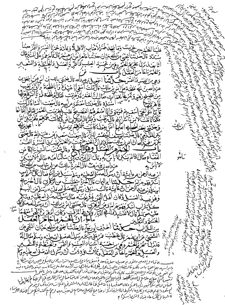
This method focuses on special manuscripts pages containing skewed notes. These notes are mainly written by students studying these manuscripts a thousand years ago. Due to this, the manuscripts now contain several texts written by different people, and the notes part is mostly written around the main text resulting in skewed lines.

You can download the data from here.

Gabor Filter Bank¶

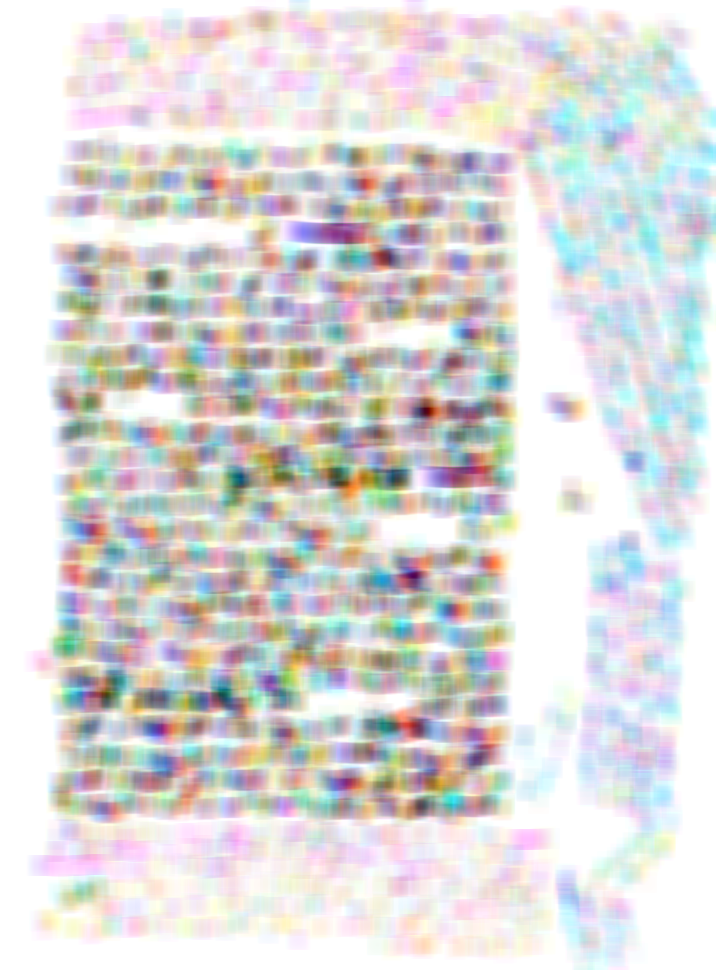
Instead of feeding the grab-cut algorithm the original image, we provide it, as input, an RGB image created from the Gabor filter bank.

The two-dimensional Gabor transform is defined as follows: \begin{equation*} \begin{split} g(x,y) = \exp(-\frac{x'+\gamma^2y'^2}{2\sigma^2 })cos(2\pi\frac{x'}{\lambda}+\psi) \\ \\ Where: x' = xcos(\theta) + ysin(\theta) \\ y' = ycos(\theta) - xsin(\theta) \\ \end{split} \end{equation*}

The Gabor transform parameters, and values used:

$\psi$ is phase offset - set to zero.
$\gamma$ is standard deviation of the Gaussian - set to 1.
$\theta$ is the orientation of the Gabor transform - three values:
- $\frac{\pi}{4}$ - down-right to top-left
- $\frac{\pi}{2}$ - down to up
- $\frac{3\pi}{4}$ - down-left to top-right
$\lambda$ is the wavelength of the cosine factor - see below
$\sigma$ is the spatial aspect ratio of the Gabor function - set to 1.

The wavelength of the cosine factor is determined as follows:

\begin{equation*} \begin{split} F_{L}(k) = \frac{1}{4} - \frac{2^{k-\frac{1}{2}}}{w} \\ \\ F_{H}(k) = \frac{1}{4} + \frac{2^{k-\frac{1}{2}}}{w} \\ \end{split} \end{equation*}

Where:

$k=1, 2,..., \log_{2}^{\frac{w}{8}}$
$w$ is the width of the image

On the output of each application of Gabor transform, we apply a non-linear function as follows:

\begin{equation*} tanh(\alpha t) = \frac{1 - e^{-2 \alpha t}}{1 + e^{-2 \alpha t}} \end{equation*} Where:

$\alpha = 1/4$
$t = 1$

Finally, we apply Gaussian smoothing on the results, where $a = 3$, and $b = 1$.

Gabor Filter Bank - C++ Code¶

After the mathematical introduction, now we will look at the code of these equations. The code implementation can be found in marginalnotesdetection.cpp file, function createGaborBank().

Creating Orientation Array - $\theta$¶

We will begin with $\theta$ values and create an array for them. Please note that their quantity can be easily changed following your liking. We've used three values of theta in our case to generate an RGB matrix (channel for each theta).

ORIENTATION_COUNT = 3; // number of orientations (theta values)
QVector<double> thetas; //the orientation of the filter

for (size_t i = 0; i <= ORIENTATION_COUNT; i++) 
	thetas.push_back(i * M_PI / 4); //M_PI is pi

Calculating Wavelength of sinosoidal factor - $\lambda$¶

Next, we will calculate the values of the sinusoidal factor wavelength.

//calculating lambda's values // wavelength of sinusoidal factor
QVector<double> J;
for (size_t i = 0; i <= std::log2(fImage.cols / 8); i++) {
	J.push_back(0.25 - ((qPow(2, i) - 0.5) / fImage.cols));
	J.push_back(0.25 + ((qPow(2, i) - 0.5) / fImage.cols));
}

QVector<double> F;
for (size_t i = 0; i < J.size(); i++) {
	double min = DBL_MAX;
	int minIdx = -1;
	for (size_t o = 0; o < J.size(); o++) {
		if (min > J[o]) {
			minIdx = o;
			min = J[o];
		}
	}
	F.push_back(J[minIdx]);
	J[minIdx] = DBL_MAX;
}

QVector<double> lambdas;
for (size_t i = 0; i < F.size(); i++) {
	lambdas.push_back(1.0 / F[i]);
}

Gabor Filter Bank¶

Using three orientations, and 14 different wavelengths, we end up with 42 Gabor responses which will denote our filter bank. The array fGaborFilterBank will store the 42 Gabor responses. For each orientation, we combine the response matrices received from the filter, resulting in one matrix per orientation. By merging them together we end up with an RGB image showing the result.

int kernel_size = 9; // size of filter 
double sigma = 1; // standard deviation of gaussian envelope
double gamma = 1; // spatial aspect ratio
double psi = 0; // phase offset 
                // 0 is the real parts of the gabor filter 
                // pi/2 is the imaginary parts 

//Step 1: Gabor Filter Bank Generation
//now we generate the gabor filter bank from the parameters                
for (double theta : thetas) {
	cv::Mat matToPush;
	int idx = 0;
	for (double lambda : lambdas) {
		cv::Mat dest;
		cv::Mat kernel = cv::getGaborKernel(cv::Size(kernel_size, kernel_size), 
                                            sigma, theta, lambda, gamma, psi);
			cv::filter2D(src_f, dest, CV_32FC1, kernel);
		cv::Mat dest2;
		if (idx == 0)
			matToPush = dest;
		else
			matToPush += dest;

		idx++;
	}
	cv::Mat dst;
	fGaborFilterBank.push_back(matToPush);
}

Applying non-linearity and Smoothing¶

Two steps left to do after generating the Gabor responses. We need to apply a non-linearity function, and afterwards a smoothing function. For non-linearity we apply tanh, and for smoothing, we use Gaussian filter.

//Nonlinearity
for (cv::Mat entry : fGaborFilterBank) {
	for (int i = 0; i < entry.rows; i++)
		for (int j = 0; j < entry.cols; j++)
			entry.at<float>(i, j) = std::tanh(0.25*entry.at<float>(i, j));
}

//Smoothing
double b = 1;
for (size_t i = 0; i < fGaborFilterBank.size(); i++) {
	cv::Mat dest;
	cv::Mat dst;
	double lambda = lambdas[std::floor(i / thetas.size())];
	sigma = 3 * ((1 / M_PI) * 
                    std::sqrt(std::log(2) / 2) * (qPow(2, b) + 1) / (qPow(2, b) - 1) * lambda);
	cv::GaussianBlur(fGaborFilterBank[i], dest, cv::Size(2 * std::floor(sigma) + 1, 
                                                         2 * std::floor(sigma) + 1), sigma);
	fGaborFilterBank[i] = dest;
}

Results¶

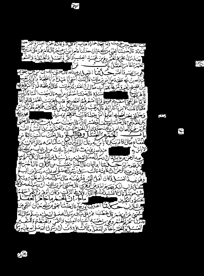
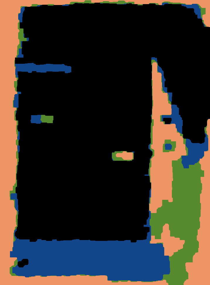
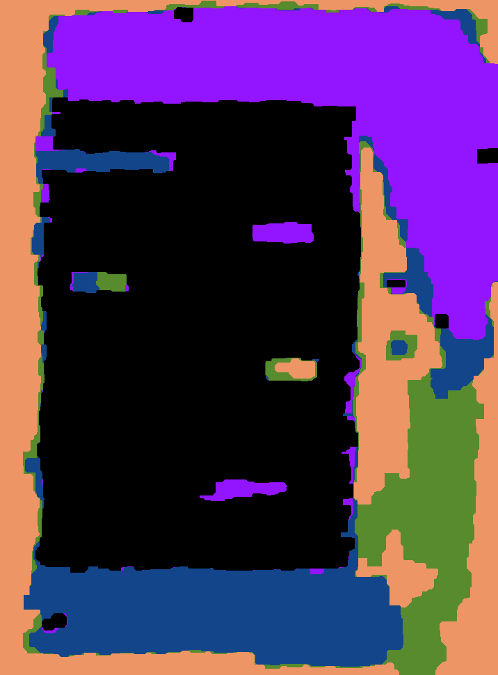
The first row of the images illustrates what the user sees when executing an interactive layout segmentation of a manuscript. Starting with left most image showing the manuscript page, and moving right each time shows one segmentation of page. Each time it segments and removes one paragraph of the manuscript page.

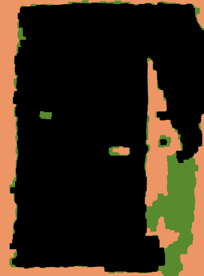
The second row illustrates what happens behind the scenes. Starting with the left most image showcasing the RGB image of superimposing the Gabor responses. Each image to its right shows the generated mask, where each stage is colored differently. The colors denote the paragraphs detected in the interactive segmentation process.